Dynamic Characteristics of German HBM Sensors

In actual measurements, the input of the German HBM sensor may be a continuous signal with rapid changes, or it may be an impulsive or periodic input. At this point, the characteristics represented by the transient processes caused by various types of energy storage components in the sensor are significantly different from the static characteristics. The relationship between output and input will be a function that varies over time. Therefore, it is necessary to study the dynamic characteristics and indicators of sensors.

The description and analysis methods for the dynamic characteristics of German HBM sensors are the same as those commonly used in general control systems, but the focus is different. In general, a sensor can be regarded as a dynamic replication system, and the requirement for this system is to replicate the input effect with minimal error under dynamic operating conditions (input is a function of time variation).

2.3.1 Relationship between frequency characteristics and dynamic quality

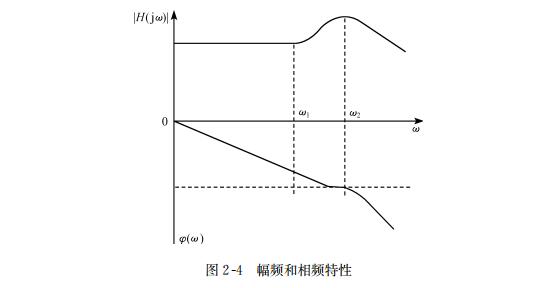
The ratio of output amplitude to input amplitude of a linear system under sinusoidal input is called the amplitude frequency characteristic of the system, represented by | H (j& omega;) |, while the phase characteristic between input and output that varies with frequency is called the phase frequency characteristic, represented by& Phi; (& omega;) represents. Figures 2-4 show a typical amplitude frequency and phase frequency characteristics, collectively referred to as frequency characteristics.

The frequency characteristic is a very useful evaluation characteristic of German HBM sensors, used to evaluate the replication error of sensors under complex waveform periodic input.

Theoretical proof shows that in Figure 2-4, the amplitude frequency characteristic exhibits a linear interval of 0<& Omega; ＜& Amp; Omega; 1. Due to its flat amplitude frequency characteristics, it has the same sensitivity to all harmonic inputs falling within this range, thus generating no amplitude error. The phase frequency characteristics of linear variation can ensure that any complex waveform composed of various harmonics that do not appear can be accurately reproduced. From this, it can be concluded that the shape of frequency characteristics is of great significance for evaluating dynamic errors.

It can also be proven that if the natural frequency is widened, the flat range under the specified accuracy will also be widened. Therefore, by changing the natural frequency of the sensor, the dynamic range can be changed.

Finally, there is a definite relationship between frequency characteristics and time response, and transient response can be calculated through frequency characteristics. From the frequency characteristics of typical links, the influence of structural parameters on it and the relationship between transient response can be understood.

1. First order German HBM sensor

Sensors with simple energy transformation, such as most physical sensors, can have dynamic performance described by first-order differential equations. By directly using differential equations or transfer functions, the frequency characteristics of typical first-order sensors can be obtained, namely

The corresponding amplitude frequency and phase frequency characteristics are

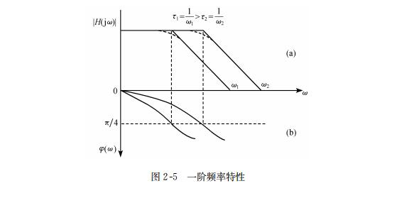
The graph is shown in logarithmic coordinates in Figures 2-5. From the figure, it can be seen that the first-order frequency characteristic has the simplest form, and its characteristic parameters can be obtained from the 3dB frequency; Omega; C represents, i.e

Here,& Tau; It is called the time constant of the sensor. As shown in the figure, the time constant& Tau; The smaller, the 3dB frequency; Omega; The higher the c, the better the dynamic response. Alternatively, smaller time constants respond faster.

2. Second order German HBM sensor
　 　 　 　 　 　 　 　 　 　 　 　 　 　 　 　 　 　 　 　 　 　 　 　 　 　 　 　

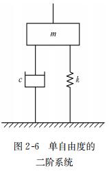
As is well known, circuits with R, L, and C in electrical systems exhibit second-order frequency response. Similarly, mechanical systems with damping, mass, and springs (Figure 2-6), such as sensors for measuring force and vibration, also have similar characteristics. According to the principle of force balance, differential equations can be listed

From this, the frequency characteristics can be obtained

In the equation,& Chi; Is the frequency ratio,& Chi;=& Amp; Omega;/& Amp; Omega; 0& Amp; Omega; 0 is the natural frequency of the system without damping,& Amp; Zeta; Is the specific damping coefficient, 。

The amplitude frequency and phase frequency characteristics can be obtained from equations (2-8), and their corresponding graphs are shown in Figure 2-7.

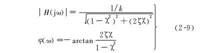
As shown in the figure, the frequency characteristic is related to two parameters, namely the undamped natural frequency; Omega; 0 (at& chi;=1) and specific damping coefficient& Zeta;, At the same time, it can be seen that the magnitude of the resonance peak and the resonance frequency& Omega; N With& Zeta; By differentiating equation (2-9) and making it equal to zero, we can obtain

　 　 　 　 　 　 　　

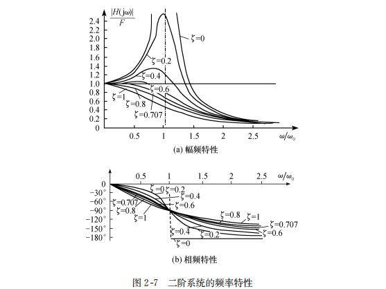
From this, it can be seen that in& Zeta; ＜ At 0.707, at a certain& Omega; Resonance occurs at 0. On& Zeta;= At 0.707,& Omega; If n=0, the resonance peak will no longer appear, and this state is called the critical damping state.

From both graphics and calculations, it can be shown that the frequency characteristics of second-order systems can be represented by two characteristic parameters& Omega; 0 and& Zeta; To evaluate: on the same& Zeta; Below,& Omega; The larger the 0, the larger the flat area of the characteristic, and the better the dynamic characteristics; At a certain natural frequency, when& Zeta;= At 0.707, it has the widest amplitude frequency characteristic flat region.

2.3.2 Time domain response characteristics and dynamic quality indicators

Analyzing dynamic response characteristics in the time domain is an intuitive method that can provide clear concepts for evaluating dynamic errors. Under the action of rapidly changing inputs, the relationship between the input and output of the sensor is a time-varying one. The reason for this phenomenon is the influence of transient components of the system caused by input effects. Therefore, the output of the system under dynamic conditions can be seen as composed of two components: the first component maintains a definite relationship with the input like a static characteristic; The second component is the transient component caused by input action, also known as dynamic error.

Obviously, the transient component reflects the dynamic balance between the process of energy storage (electric field, magnetic field, potential energy, kinetic energy, and heat accumulation) and the process of consumption (resistance, friction, etc.) in the sensor. By using typical input actions, the relationship between them can be observed, and the most commonly used typical input action is the step function. Figures 2-8 represent representative step response curves under zero initial conditions. In the figure, y (& infin;) represents the steady-state value after the transient ends, and its relationship with input x (t) is determined by the static characteristics. From the figure, it can be seen that the influence of transient components is only displayed in the front part, so the dynamic quality parameters of the sensor can be represented by certain features of the front part of the step response, commonly used as follows (Figure 2-8):

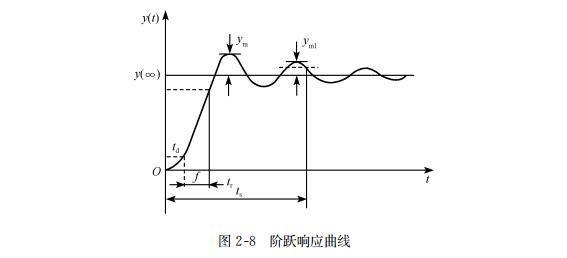
① Time delay. The time interval from the step input to the change in output response, expressed in td.

② Rise time. To eliminate the influence of time delay, the starting point of the rise time is set at the point where the output response reaches a certain percentage point (5% or 10% of the steady-state value), and the endpoint is at the point where the output first reaches a certain percentage point (such as 90%) of the steady-state value. Obviously, this time interval is related to the two specified percentages, represented by tr, and the corresponding percentages are given.

③ Step response time. The time required for the output value to reach the specified error range of the steady-state value for the first time starting from the step input, often expressed in ts, and given together with the specified error, such as ts (5%). Obviously, ts includes time delay.

④ Instantaneous overshoot. For step response, the output value exceeds the maximum instantaneous deviation ym of the steady-state value, and this deviation is expressed as a percentage of the steady-state value, such as。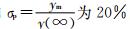

⑤ Attenuation. Used to describe the rate of step response attenuation of oscillations, in& Phi; Represent. Its value is expressed as the percentage of the difference in amplitude between adjacent overshoots (ym1-ym2) and ym1,& Phi; The larger the value, the faster the attenuation.

⑥ Stable time. It describes the entire time from the beginning to the end of the transient process, represented by ts1. To specify the end of the transient (which may theoretically take infinite time, a steady-state errorε needs to be specified. The stability time is the time required from the step input to the output response finally entering the specified error range.

As can be seen from the above, the dynamic performance of German HBM sensors can be described by one or several parameters. The description method is related to the characteristics of the transient process of the sensor. For example, the description of monotonic processes and decaying oscillation processes may differ greatly. Below, we will discuss two typical processes based on the characteristics of transient processes.

1. Step response of monotonic changes

An open-loop system composed of multiple inertial links has a monotonic step response, and its performance can be described by one of three factors: rise time, step response time, or stability time. For a simple system with only one inertial link, the step response can be immediately and completely determined by providing a time constant, as shown in Figure 2-9

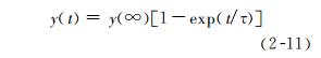
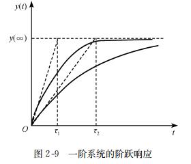
As shown in the figure,& Tau; The smaller the response time and stability time, the better the dynamic performance. Compared with equations (2-6), it can be seen that& Tau; Small means wider frequency bands.

2. Typical second-order systems

The transfer function of a second-order system can be obtained from equations (2-7), namely

Figure 2-10 shows the step response curve of the second-order system, where& Zeta;= The curve of 0.707 represents the critical damping state. By comparing the three curves, it can be seen that the critical damping has the minimum stability time; Zeta; The smaller the value, the shorter the rise time. From the perspective of response time, critical damping is not the optimal state. Analysis shows:& Zeta; The smaller the value, the greater the instantaneous overshoot. Therefore, in practice,& Zeta; 0.5 to 0.7, in order to obtain the minimum response time under allowable overshoot conditions. Comparing Figures 2-7 and 2-10, it can be seen that the smaller& Zeta; The value has a wide bandwidth (3dB), so the rise time is related to the bandwidth.

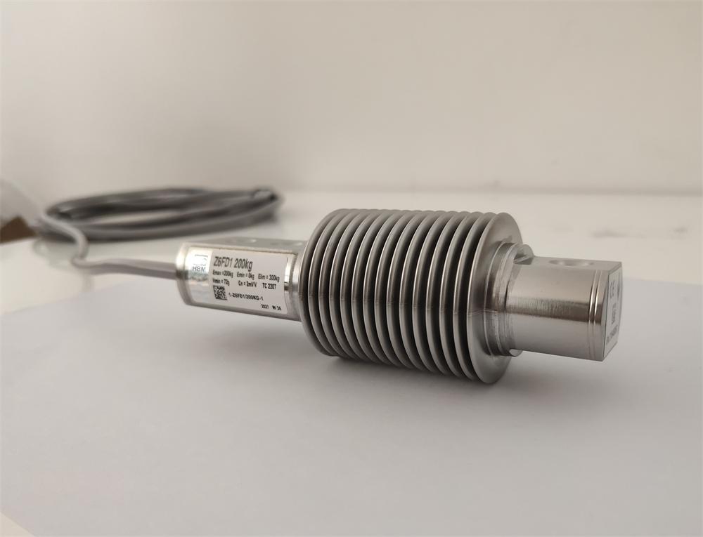
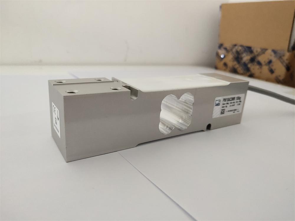
★German HBM: Load cells - Series Z6F, C16I, C16A, RTN, HLCB1, PW2D, PW6D, PW2C, PW6K, PW6C, PW10A, PW12C, PW16A, PW22, S40A, C2, etc
★　German HBM: Torque/force sensors - T40B, T22, T5, U9C, C9C, S9M, U2B, S2M, and other series
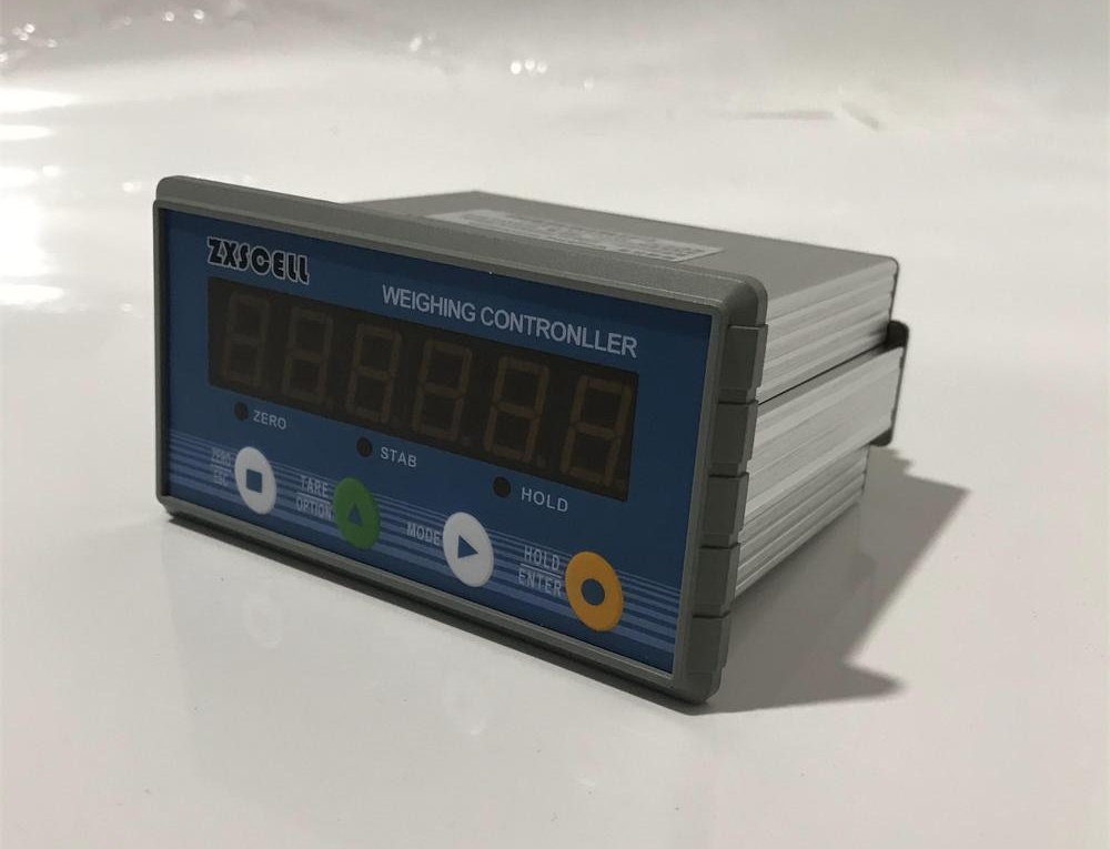
★　German HBMWeighing instruments/transmitters - WE2111, RM4220, BM40, AE101, AE301, EM201 and other series
★　American CeltronSensors - STC, HBB, LPS, LOC, PSD, LCD, MBB, SQB, and other series
★ Tedea huntleigh: --341061635510151040102212601201241240 and other series
★　American TranscellSensors - BSS, BSH, DBSL, SBST, CR, SBS, BAB, and other series
★　Mettler Toledo: Load cells - TSC, TSB, MTB, GD, SLB415, SLB215, MT1022, MT1260, MT1241, SB, SBS, SBH, and other series
★ METTLER TOLEDO: Digital Sensor& Flash; GDD, SLC7200760, PDX, SLC820 and other series
★ Mettler Toledo: Control instruments - IND331, IND245, IND320L, IND230, IND560, B520, IND110, WM0800, AJB and other series
　
Contact person: Huang Hao Tel: 18688492451 (WeChat with same phone number)